In this post, I’m going to make the perhaps provocative claim that some of the Bitcoin HODLers are operating under a false dichotomy: It seems they think that if you really believe in the long-run performance of Bitcoin, that you shouldn’t worry about “hedging downside risk” and should go “all in” right away. In this mindset, any temptation to occasionally rebalance your portfolio with some allocation to a safe(r) asset is an implicit admission that you don’t have the stomach for Bitcoin.
In contrast, I am going to argue that even in the very long run, you will end up holding more satoshis if you include at least a small allocation to a safer asset, and periodically rebalance your portfolio. To repeat, I am NOT merely talking about smoothing out the volatility to limit your downside exposure along the way. I am making the stronger claim that even if your single-minded goal is to maximize the expected long-run growth rate of your portfolio, a 100% allocation to Bitcoin is not necessarily optimal.
In the present post, I’ll start with a simple coin-tossing example to motivate the distinction, and then I’ll dive into a Monte Carlo simulation of Bitcoin runs over the next ten years to make my point concrete.
A Coin Tossing Example
Suppose you put up $100 on a single coin toss. If it comes up Heads, you are paid back $150. If it comes up Tails, you are paid back $60. Should you play this game?
The answer is “yes,” at least if you have some wealth. The mathematical expectation is that you will win $5 with each play. (There’s a 50% chance of winning $50 and a 50% chance of losing $40.) No casino would host such a game, because over time they would lose money.
However, if you are allowed to keep playing this game many times in a row, you would not want to keep “letting it ride.” To see this, consider that in a typical sequence, where the player has 1 win and 1 loss, his return is +50% and -40%, which in multiplicative terms is (1.5) x (0.6) = 0.9. In other words, starting with $100, the player will end up with $90 if he plays the game twice in a row, and either has a H-T or a T-H sequence. (Specifically, he might go $100->$150->$90, or he might go $100->$60->$90.)
I won’t dwell on the more sophisticated mathematical treatment here, but suffice to say, the difference in the two approaches related to the arithmetic mean versus the geometric mean. The standard assumption in introductory economics and finance courses is that we deal with uncertainty by taking an average of the possible outcomes, weighted by their probability of occurrence. As this simple example shows, we need to be careful about what “average” we have in mind.
I hope this simple example has intrigued you enough to consider the application to Bitcoin. What I’ve shown above is that even if you have a game with a positive expected payoff, because of the volatility in the returns, it’s not optimal to bet your entire bankroll with each play of the game. If you want to see more analysis on this particular example, see my earlier blog post, which gets into the so-called “Kelly criterion” of optimal bet sizing in such a framework.
But now let’s apply this idea to the case of Bitcoin.
A Monte Carlo Simulation of Bitcoin
I did a quick and dirty simulation just to motivate this idea. As I get feedback from the HODLing community, I can refine my presentation. But for our purposes right now, here’s what I did:
I am modeling a 10-year horizon of Bitcoin returns, where things are updated monthly. I enter an initial Bitcoin spot price of $85,000, and a target future price (in 10 years) of $850,000. This implies a compound annual growth rate (CAGR) of 25.9%. I also set the dial to a Bitcoin volatility of 80%, which in this context is the standard deviation of the annual log returns, which we assume are normally distributed. (To make it concrete: This means that about 68% of the time, Bitcoin’s annual return is plus or minus 80% around the expected return.)
Then, I run 1,000 simulations of hypothetical Bitcoin price trajectories with these characteristics. I report those results. Notice that the median Bitcoin price after 10 years will not necessarily be close to $850,000, because these are random outcomes. However, I kept redoing the analysis until I got an outcome where the median Bitcoin price after ten years was in fact close—in this case, about $839,000.
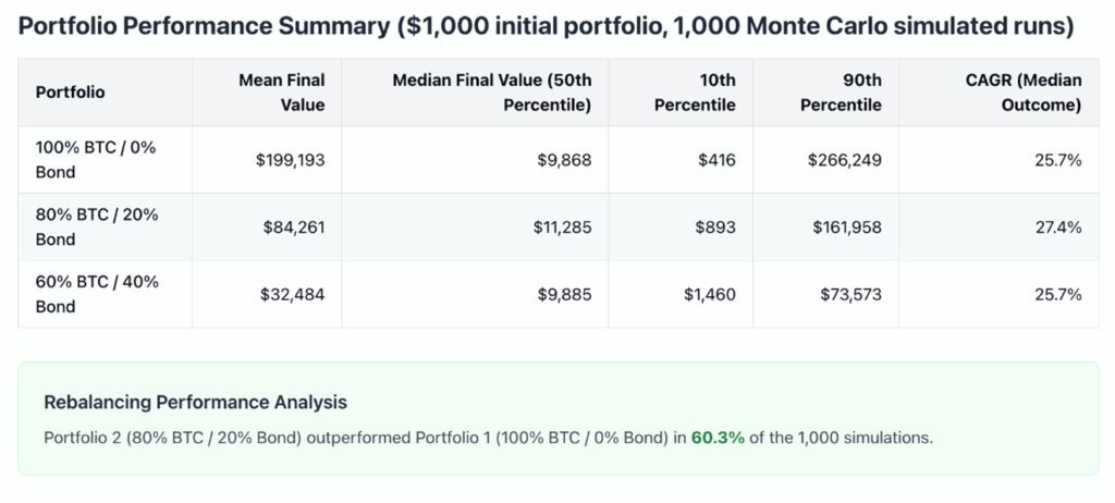
Finally, I showed three model portfolios starting with $1,000 each. The first portfolio is straight HODL. The second is 80% Bitcoin and 20% bonds (which we assume grow at a constant 4% annualized return). The third is 60% Bitcoin and 40% bonds.
We rebalance monthly. So if the Bitcoin price has recently spiked, then a higher fraction of the portfolio is in Bitcoin than desired, so some of the Bitcoin is sold for dollars which are used to buy more bonds. On the other hand, if Bitcoin should crash, then in the next rebalance, some of the bonds are sold off and the money is used to buy more Bitcoin (at the low price).
Then we report the performance of these three model portfolios after the ten years.
The Results


Some observations on the above results:
First, notice that with our assumptions, the final price of Bitcoin after ten years is incredibly open-ended. In the worst scenario of the 1,000 simulated runs, Bitcoin ended the decade at a mere $384. In ten percent (i.e. 100) of the 1,000 runs, Bitcoin ended at $35,375 or less. On other hand, in the best run, Bitcoin ended at $1.8 billion. In the best 100 of the runs, it ended at $22.6 million or higher. And the median outcome was $838,785. (Notice that the mean outcome—which is the arithmetic average over all 1,000 simulated runs—is much higher, at $16.9 million. That’s because the few outcomes with outrageously high performance are swamping the more likely, mediocre outcomes.)
Given this incredible range of possible Bitcoin performance over the hypothetical decade, we see different returns on our model portfolios, which (remember) all start at $1,000. The pure HODL portfolio has a mean final value of a whopping $199,193. But that is driven by a small number of explosive trajectories. The median outcome is $9,868, which implies a CAGR over the period of 25.7 percent. (Notice this is very close to our parameter setting which implied a Bitcoin CAGR of 25.9%.)
In contrast, the more conservative portfolio, which every month rebalances to maintain 80% allocation to Bitcoin and a 20% allocation to the safe bond, outperforms if we look at the median performance. Specifically, in the median outcome the 80/20 portfolio has a final value of $11,285, implying a long-run CAGR of 27.4%.
The final point I wish to stress is that we are not here merely talking about anxiety reduction. I am not simply saying, “Hey, if you are faint of heart and don’t like roller coasters, maybe you should mix in some bonds to your portfolio.”
Rather, I am arguing that even if all we care about is the final market value, after a pretty long time horizon—in this case, ten years—it is still the case that the 80/20 portfolio beats the pure Bitcoin portfolio in 603 of the 1,000 simulated runs. So even if you want to maximize the number of satoshis you own at the end of Year 10, and you don’t care at all about the ups and downs in between, in 60.3 percent of the runs, you would be able to cash in your bonds and buy more bitcoins at the very end, to have a higher “score” with the 80/20 portfolio, rebalancing every month along the way.
Now to be sure, you would get different results by fiddling with the parameter choices. But I hope I’ve at least gotten the reader to consider that pure HODLing might not be the best strategy, if you think that Bitcoin will experience large volatility along with its high average returns, over the coming years.
Dr. Robert P. Murphy is the Chief Economist at infineo, bridging together the dependability of Whole Life insurance policies with the benefits of blockchain-based finance.
Twitter: @infineogroup, @BobMurphyEcon
Linkedin: infineo group, Robert Murphy
Youtube: infineo group
To learn more about infineo, please visit the infineo website

